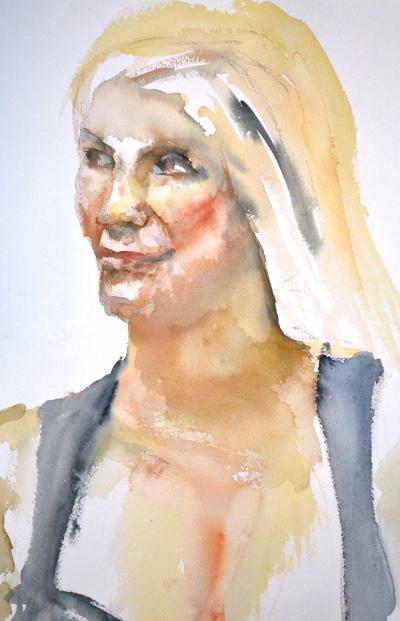
Start of aquarelle painting season 2019 - 2020 Thursday, 12-Sep-19 08:05:00 CEST

An Aquarelle Portrait of Tasha Thursday, 19-Sep-19 21:30:36 CEST

Saturday, 14-Sep-19 06:50:34 CEST

Learning Machine Learning and Artificial Intelligence, Part 2

Tuesday 3 September 2019

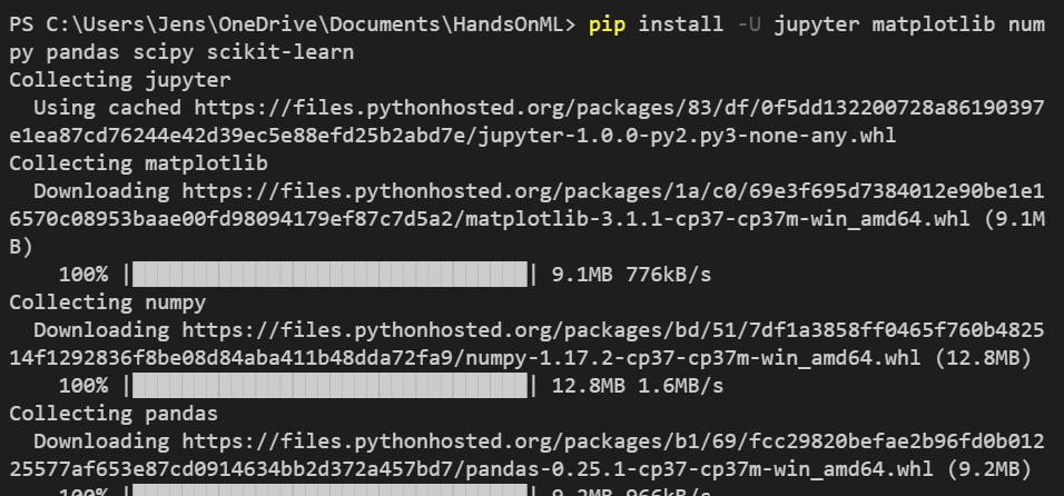
This is part two of my journey learning Machine Learning and Artificial Intelligence with the book Hands-On Machine Learning with Scikit-Learn & TensorFlow by Aurélien Géron. In my previous post in this series, I talked about how I found this book and started reading it. I covered the first two chapters. I am reading the book, trying the exercises and thinking out loud here in the blog what I find in the book. In my blogs, there are also snippets of other parts of my life, such as the creation and building of our new house.

Today I received a message from the municipality that I had to fill in another form about where I get my money from to build the house – they call it the “Bibob” form. Well, it is simple, I work to get money, and I borrow my money. No, Jens, for the municipality it is not that easy. Eight pages of stuff to fill in. Well, not tonight.

I am on page 88 of the book, section Precision, and Recall of chapter 3.

So if the diagonal from the upper left and bottom right got high values, the classifier is doing a great job, and one way of measuring that is with the help of a formula. The f1 formula.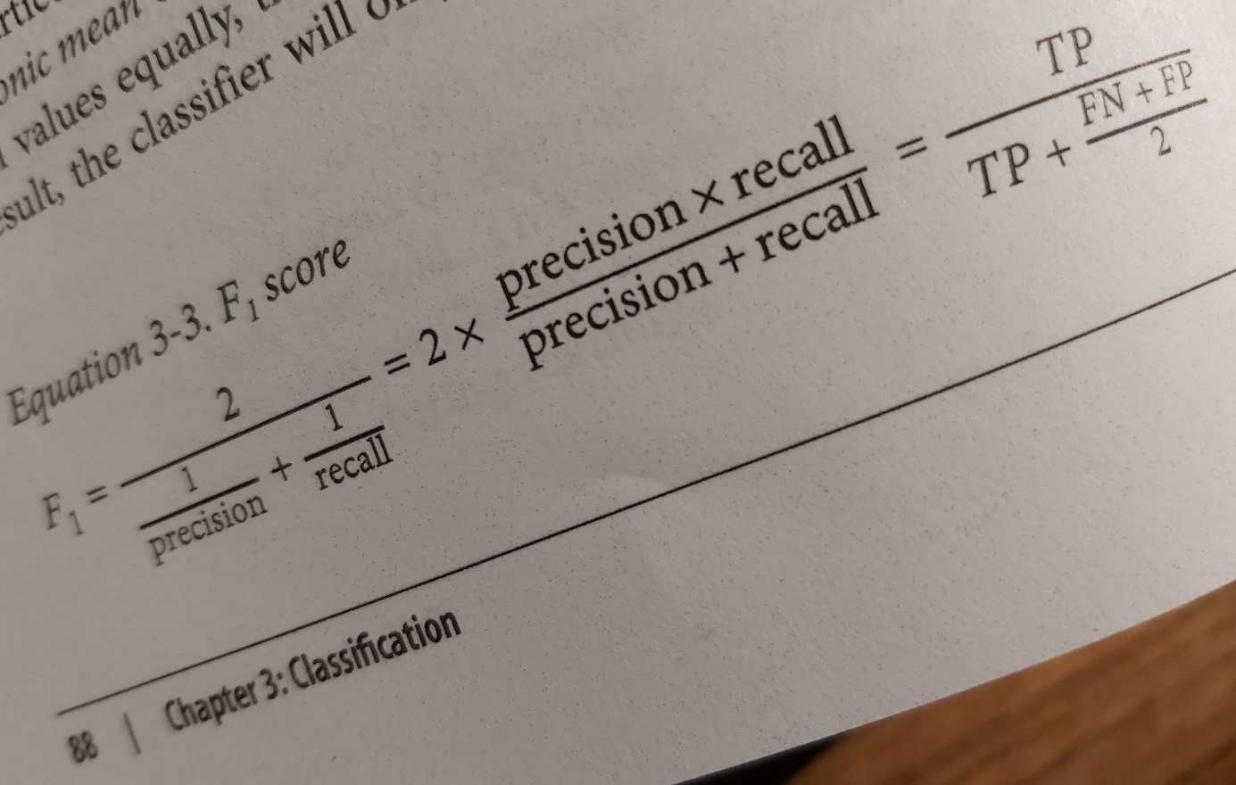

Almost like a given this is already figured out in the SciKit learn library. Just call the f1_score() function.

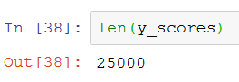
The book then goes on talking about how the precision and the recall can be an instrument for gaining understanding about how good the algorithms are working. Then they are making a graph with this.

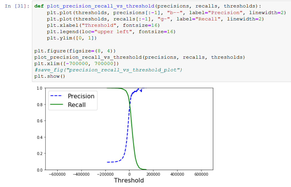
I like graphs, so I had to print it as well. I did not have so much data because I only got 32 bit Python installed. I changed x-limit.

Now my graph looks similar to the book.

Bedtime! Bye.

Thursday 4 September 2019

I have been thinking about how we got from the Confusion Matrix via Precision/Recall to the graph. It puzzled me. I have a faint idea of how this goes, and I will explain it to myself in here in a way so that I understand it. We take it in small steps.

There is a kind of black box that we can use to classify an image. That is SGDClassifier.

We will evaluate the performance of the classifier with the help of the confusion matrix. The image stored in the variable “Some image” is what we are looking for – it is a 5, and all other cases are non-5. We get counts of four possibilities such as True Negative (Good), False Positive (Bad), False Negative (Bad) and True Positive (Good). With many good compared to fewer bad answers, that might be what we are looking for.

Precision is the counts of TP / (TP + FP). It is the counts of TP that we desire to find in relation to the total of both TP and FP. Recall TP/ (TP + FN) is the counts of TP we desire to find in relation to the total of both TP and FN. The FN count is the number of images that we ought to find, but they were incorrectly left out. They should be classified to be 5, but they were not. They are missed. This relation is looking at all that should have been 5 FN + TP and this in relation to the TP. Perhaps this just needs to sink in.

Anyhow from here, we get that there is a tradeoff between precision and recall. One cannot have both. They are each other's opposite.

A classifier is using various techniques to figure out if the lumps of pixels is a five or not. It is not deliberately making false negatives. The false negatives are the result of that algorithm. But something in here makes it possible to skew the behavior of the classifier so that we get more recalls than precisions and vice versa.

Here we come to the core of what I had troubles understanding. The classification algorithm in itself is not aware of any precision or recall. Or is it? It is just taking pixels and deciding what number it should represent.

At the top of page 90, we are told you can use the decision function method. It can return the score of each instance. That score is the harmonic mean value they talked about on page 88. So with that, we get a number indicating the relation between precision and recall.

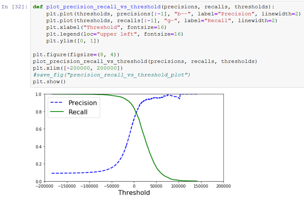
I suppose we can run the prediction over and over again, and each time we store the score, precision, and recall. When printing this in a graph, it looks like this (in my case).

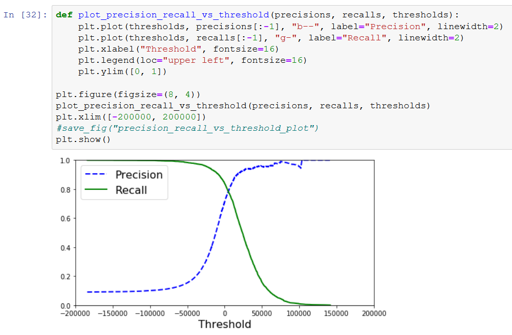
So the x-axis is the score. When precision is low, the recall is high. Somewhere at 0 precision and recall are meeting.

I think this stuff got a place in my brain now and that will have to do for now. Tomorrow night I will go to the start event of the aquarelle painting club so I will not have any time for AI and ML tomorrow evening.

Good Night.

Friday 6 September 2019

Yesterday evening I went to the first aquarelle club gathering for this season. We looked at a video by Shirley Travena. It was nice. We talked about Shirley's painting techniques, had coffee, and caught up on what had happened since the end of the previous season.

Tonight I have one hour for AI/ML. I am on page 92 and just about to look into a diagram plotting precision against the recall.

I just want to say something first. This is really not what I had expected by this book. Obsession with measuring how good something works, so much so that it is not even explained how things are done before we measure how good they are. I am using a stochastic gradient descent classifier, and I have no idea what it is.

My son is studying computer science at the uni, and we talked about the difference in how he is studying and how I am studying. I said to him that he should learn in a way that he can produce sufficient result at the exam. I, on the other hand, is learning because I want to use this stuff.

Anyway. Let us move on. On page 90, there is the sentence “Scikit-learn does not let you set the threshold directly,” and on page 92, the book says, “…just set a high enough threshold.” I am confused here, but I am leaving this now.

The book has a graph plotting the recall against the precision, but it is not telling how to get it. From the GitHub, I can see how the writer did it.

https://github.com/ageron/handson-ml/blob/master/03_classification.ipynb

At step 41. Cannot find this in the book.

That is so much of Python magic. What is going on here?

I went on a little detour on my own to decipher this. I entered y_scores in a cell and evaluated that.

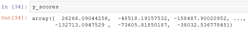
It is an array of numbers, the y_scores. How many of these?

25 thousand. All right. So what happens when you take an array like that and do it more than a number?

You get 25 thousand trues and falses. This is good fun. Here I am getting to the core of something. Let us continue.

So what is the train predictions?

Okay, so an array of Booleans equal to another array of Booleans gives a new array of Booleans?

Indeed it does. So what is up with the all() function?

A google search tells me that if all elements are true, then all return true. Now we can translate the Python statement to natural language.

So the scores more than zero is identical to the predictions. Ok. Fine.

I will find out how to make graphs like this. Great fun!

Obviously, I don’t have the save fig routine. I might have missed that somewhere. It is not in the book. Since I can see the graph on the screen, I don’t need it.

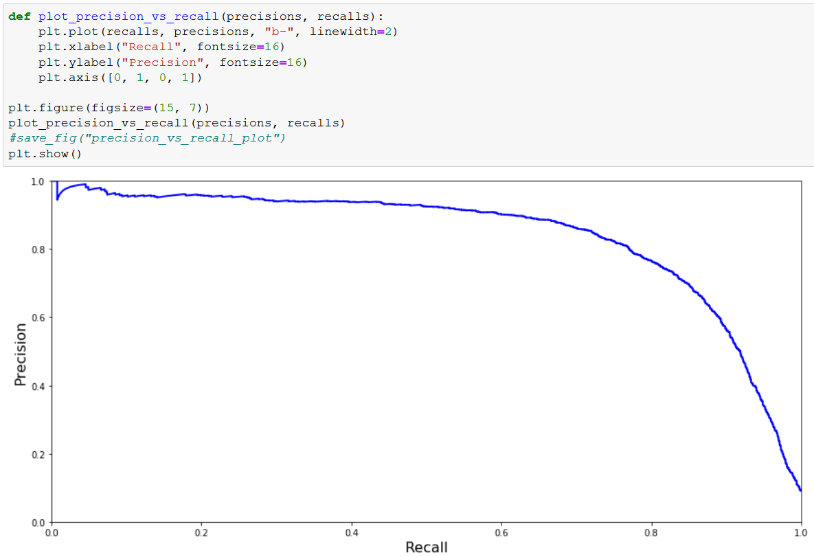
Now we are going to the ROC curve on page 93.

Sunday 8 September 2019

It is already Sunday, and I am about to blog a little bit about ML and AI. Yesterday we finished the Bebop form. I will submit it to the municipality on Monday.

Now we will plot another curve describing the quality of classifiers: The Receiver Operating Characteristic (ROC) curve.

I read the text, and I cannot make any conclusions about it. Here is what I am seeing.

So by reading this, I try to figure out the formula for True Negative Rate.

How difficult can it be to present the names and formulas of things without messing up? If you write a book about complex things, please just present the terminology in a way that it is easy to understand. If we need to understand 4 things, then mention these things one after another. Don’t leave it for the reader to clear up your mess, dear writer. You don’t write a blog, that is what I am doing. You write books. Do it right.

I cannot see there is a formula for the TNR on page 93. There is a sentence, though. It says that TNR is the ratio of negative instances that are correctly classified as negative. So if “negative instances” refer to the entire upper row of the confusion matrix and “correctly classified as negative” is the TN part of the upper row. That could give a formula for TNR to be TN / (TN + FP).

Started making a table of what I learned so far and my guesses. Then I started to google for better explanations. Here is a link to a page that is doing this explanation much much better than the book: https://classeval.wordpress.com/introduction/basic-evaluation-measures/

Precision	Recall, Sensitivity	1 – Specificity SP	Specificity SP
TP/(TP+FP)	TP/(TP+FN)	FP/(TN+FP)=1-SP	TN/(TN+FP) = TN/N
	True Positive Rate	False Positive Rate	True Negative Rate
	TPR	FPR	TNR
The ratio of negative instances that are incorrectly classified as positive.	The ratio of negative instances that are correctly classified as negative.	The ratio of negative instances that are incorrectly classified as positive.	The ratio of negative instances that are correctly classified as negative.

So this was a bad experience. I am not abandoning the book just yet though.

To get the ROC curve, I call a function for that, and the Github gives me how to plot that curve. Nice.

Aah, we are on page 94, and we will use a new classifier. This classifier is called RandomForestClassifier. Without knowing what it is, we will compare it with the SGD classifier. Good stuff. It is like having a group of children play with paint but not telling them what color it is. Then you give them another paint and tell them that now they will have to compare the two and carry out performance measurements.

This new classifier has no decision function. That was the function, IMHO that was poorly explained by the book. So this function has a predict_proba function. Normally scikit-learn has one or the other.

Here we get a row per instance and a column per class, each with the probability that the instance belongs to that class. This gives me a concrete idea about what is provided by the classifier to get an idea about the performance of the classification.

Did we have that intro section for the SGD classifier as well?

Instead of pushing ahead, I jump back to have a look for the intro to the SGD classifier. I am wondering how the book talked about the performance measurements of the SGD classifier.

Learning does not necessarily need to happen sequentially. Sometimes I skip a section and go back to it later. Here at this point, I start to understand how the performance of the classifier is measured.

I think the text on page 89 is very important, and perhaps earlier I missed that. It is the decision function. I reread my blog post, and most certainly on Tuesday 3 September, I missed the significance of page 89.

The book says: For each instance, SGD Classifier computes a score based on a decision function, and if that score is greater than a threshold, it assigns the instance to the positive class or else the negative class.

In my case, I have 25 thousand images because I installed the 32-bit version of Python. So for each of those, I get a score. If that score is higher than a threshold, then it is positive, otherwise negative. That is clear.

Another thing that I learned is that the syntax of Python can sometimes be very “dense.” It can be so compact. I am clearly not used to that, and that in combination with that the book says that scikit does not let you set the threshold directly” and then you do it yourself in your program (perhaps) that makes the confusion overwhelming.

So now we are on page 94, and that bad feeling about the decision function need to be pushed away.

And with that, it is really time to go to bed for me. It was a nice evening blogging about AI and this Hands-On book. I feel more and more frustrations with the book and the way that Aurelien Geron treats the feelings of a beginner in this field. That said, at this point, I am not giving up. Sleep well.

Monday 9 September 2019

Today I called our contact person at the municipality to ask a couple questions about our Bebop application. The work on filling in this form is not finished. I will have to add a couple of things. But first I worked at my day time job, and I came home late and started preparing a meal. While working on the meal, I decided to listen to a podcast about scikit learn.

http://traffic.libsyn.com/sedaily/scikit_learn-edited.mp3 (Machine Learning – Software Engineering Daily, with Andreas Müller, published 27 September 2016) That is now three years ago.

I started to realize several things when listening to this podcast. It was sponsored by a company providing advice for the financial sector. Hmm… that sounds like the first chapter of the book. Coincidence?

I realized that the Machine Learning and Artificial Intelligence business are booming and all sorts of people are jumping on to the bandwagon. Like I am doing and also like the writer of the book, Aurelien Geron is doing. Aurelien might not be the best person to explain scikit learn, though. There is a core team around the scikit learn library and Aurelien might or might not be part of that. That team is also focused on explaining how scikit should be used with documentation etc. It can be cool to look into that at a later stage. First, I will try to follow this book.

Ooh, they know each other. By all means, go buy it! Perhaps it is much better than this book? Please let me know, tweet about it and tag me with @JensMalmgren.

It was interesting to hear the podcast because they outlined pretty much the same steps we are learning right now for how to use scikit learn. The RandomForestClassifier was a big thing, apparently. It caused a popularity boost for scikit learn.

The scikit-learn core committer in the podcast, Andreas Müller, said they would include the capability to plot graphs of the data produced by scikit. I love that idea! Anything that can help explain what is going on inside is helpful, especially to newbies like me. A round of applause to Andreas!

So that was that. Where are we? We are on page 95.

The pages of the book taught itself how to fold to the place where I am reading right now. That is a kind of machine learning! So I thought that it would be cool to take a picture of this phenomenon and that would be it. I was wrong. I inserted this image here above. And then boom…

Haha haha

Machine learning in Microsoft Word tried to explain the picture to me. Apparently, it contains an indoor.

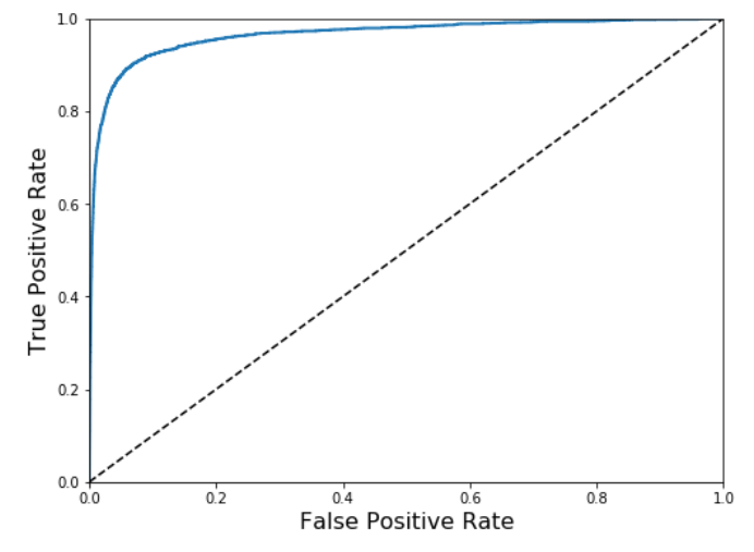
Yesterday I looked at the graph of the ROC curve, Receiver Operator Characteristic (ROC).

It has a dotted line which represents a purely random classifier. A good classifier is far away from the dotted line towards the top left corner. Good! Easy language. I can grasp this. The area under the curve AUC is a measurement of how good it is. A perfect classifier has an area of 1, and a random has an area of 0.5.

You guessed it! Scikit-learn can compute the AUC value.

I should use the Precision/Recall curve when the positive class is rare, or I care more about FP than FN. In other cases, I should use ROC.

Tuesday 10 September 2019

I am back! Last night very late, I submitted the Bibob form. It is not complete though. I will have to go to the bank to get details from them and with that my Bibob form is complete.

Here is the graph of the ROC curve comparing SGD with Random forest.

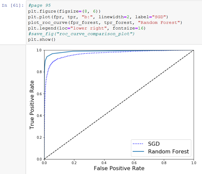
It is absolutely fantastic that you can do advanced stuff like this with a couple of lines of code.

Teased to figure out how to plot graphs. That has to wait.

The random forest classifier is much better! It comes much closer to the upper left corner.

The book for a score of .99 and I had it slightly worse.

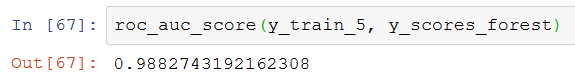
That is probably because my set is smaller.

Now we leave the classification of number five. At page 95, we embark on classifying multiple things.

There are binary classifiers versus multiclass verifiers. Up until now, we had a binary style. Now we enter the multiclass classifiers. “It is also called multinomial classifiers.” I know by now that this kind of sentences “It is also called…” at a later stage will slap you over your face so bear with me and just store this knowledge somewhere, become an academic survivor.

Ugh ugh. Aurelien, here we go again. You shuffle an incomplete table on our input bucket that we need to draw ourselves.

Classifier	Can handle multiple classes directly	Is a strictly binary classifier
Random Forest Classifier	Yes
Naive Bayes Classifier	Yes
Support Vector Machine Classifier		Yes
Linear Classifier		Yes
SGD Classifier		Yes

 

Actually here on page 96 Aurelien is not saying that the SGD classifier is a binary classifier only and he is not even mentioning it, but on page 84 the SGD classifier was presented as a binary classifier, do you remember. I had to go back to find out.

It is possible to use binary classifiers for multiple classes classification as well. If we were to classify images from 0 to 9 then we one strategy would be to have ten classifiers each taking care of a digit to see if it is that digit or not and then calculate the decision score for each and use the best. This is called the One-Versus-All(or Rest) strategy. For every classification we run ten tests I suppose.

With the next method, we compare at most two of the ten images each time. It is called One-Versus-One.

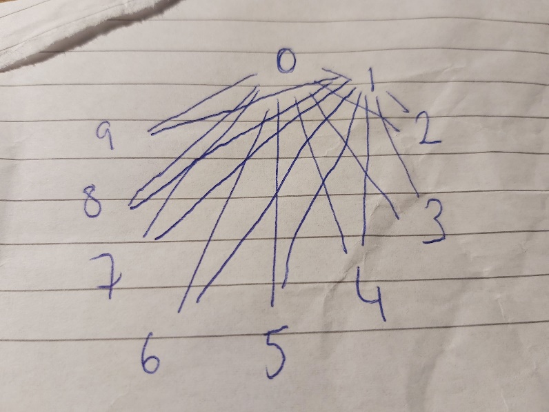
I tried to create a picture for myself how that would be done. I made a circle of the ten images. Then I drew a line from the 0 to all the rest. That was nine lines. Then I drew a line from 1 to all the rest. Also, that was nine lines. Then I stopped drawing because it would soon become very cluttered. If N is 10 in this case, then I suppose that the formula N x (N-1) / 2 pairs makes sense. So in this strategy we make, for example, a 0 and 1 classifier. I supposed. It can classify those two first images. I have no idea what happens if you come with a 2 while you have 0 – 1 classifier. Anyway, this requires that you run your images through 45 classifiers. The one with the highest score wins.

The good thing is that this One-Versus-One gives much smaller datasets to train on because it only looks at say 5 and 3 and need not know anything about all the rest.

That was it for tonight. My brain had it and need some rest. I will dream about a random forest classifier. I will envision it as a young birch tree forest.

Wednesday 11 September 2019

So this is the awful 9/11 day. I woke up in the night when my neighbor with the Harley Davidsson bike went to his morning shift. WHY DO YOU GO TO WORK WITH A HARLEY DAVIDSON BIKE IN THE MIDDLE OF THE NIGHT, ARE YOU COMPLETELY BONKERS?

Now we learned about OvO versus OvA. Here is a new version on the table I started on yesterday.

Classifier	Can handle multiple classes directly	Is a strictly binary classifier	Scalability	Preferred Multiclass Method
Random Forest Classifier	Yes			n/a
Naive Bayes Classifier	Yes			n/a
Support Vector Machine Classifier		Yes	Scales poorly on larger datasets	OvO
Linear Classifier		Yes		OvA
SGD Classifier		Yes		OvA

 

There exist a OneVsOneClassifier and a OneVsRestClassifier that presumably takes a strictly binary classifier as input and prepares it for the comparison and selection of the classification with the best score.

The book then has a section about error analysis. I read it, and I think I understand the gist of it. What's new here is that the confusion matrix is much larger. On page 86 in the first paragraph of the section confusion matrix, there is an example that much better should be here on page 98 where we can see a multiclass confusion matrix for the first time in the book.

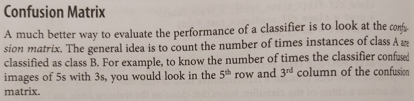
Obviously this is WRONG because what DO we find in the first row? That is the classifier data of 0s. What DO we find in the first column? That is the prediction results of the 0s. At row 6 and column 4 we find the number of times that images of 5s with images of 3s.

This snippet of text is incorrect, and it is placed at a part of the book ONLY talking about binary classifiers, so it only confuses the reader. The author should move this text to the error analysis section and fix the error. In return, he will need to write a new and better introduction to the confusion matrix.

I tried to generate the confusion matrix of the table in the book on page 98, but my 32-bit installation cannot handle it. That is not good. I start to wonder how difficult it is to install the 64-bit version, and how much will break when doing that?

I will just have to give it a go. Perhaps my Python program converting blog posts will just crash?

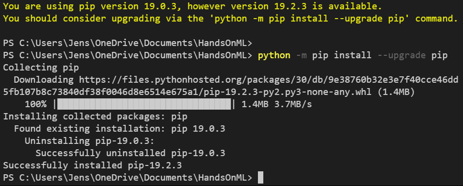
Downloaded python-3.7.4-amd64.exe.

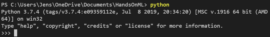
Started visual studio code.

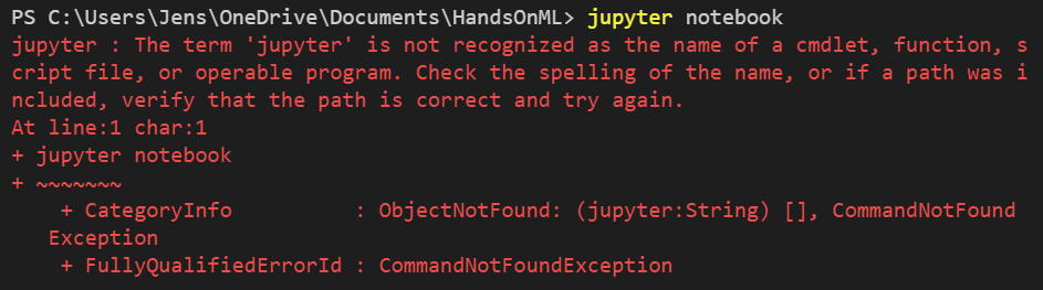
Started jupyter notebook.

Changed this from 25000.

to 60000.

As it was in the book originally.

That did not work.

Found out I had to change the system variable to the new python. The old had extension _32 and the new did not have that.

Then the new 64-bit python showed up, and I was a little bit further.

Ooh what have I done?

Perhaps I need to install that stuff again?

64 bit this time.

Then I restarted the jupyter notebook and reran my experiments, adjusting them to the original 60000 images set. Here is the cross Val score with 60 thousand images!

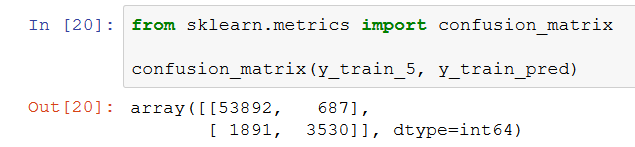
Here is the old confusion matrix with 25 thousand images:

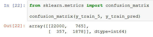
And here is it is with 60 thousand images:

Finally I came back to the place where I decided to install the 64 bit Python. The CPU is working on it now.

That took some time to calculate.

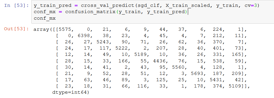
And there it is!

Thursday 12 September 2019

The book displays this matrix as a bitmap. You clearly see a diagonal. Clever. Then they divide each cell with the number of images in the corresponding class (row). That exaggerate the errors only. I like this graphic approach. The human eye can see patterns very easy compared to sifting through numbers.

The pages after the normalized error plot (100) are really good pages. Here is the first time that we get to hear how things are done inside classifier. It has been frustrating to get to this point. The SGD classifier is linear. Weights are assigned to pixels so that when there is a tiny amount of pixels with a difference, then SGD is easily confused.

Tonight I went to the first aquarelle painting session of the season 2019-2020, so this is what I do with the book tonight.

Friday 13 of September 2019

Tonight I just wrap up this chapter and post it to the blog. I hope it will work because I installed the 64-bit version of Python. The was a small easily fixed error that nothing to do with 32 versus 64 bit Python so that was nice indeed.