Our future house Sunday, 26-Jan-20 20:44:58 CET

Helen 2 February 2020 Sunday, 02-Feb-20 20:04:34 CET

Friday, 31-Jan-20 20:25:04 CET

Learning Machine Learning and Artificial Intelligence, Part 4

I hesitated if I were to publish this blog post. I decided to do it because it is part something bigger, me learning AI and ML, that is mainline in this story. The secondary storyline is the development of our future house. If you are looking for lighter reading then please read other blog posts on this site. The first half of this I

This post starts on page 124 and ends at 228. Hereby this post concludes part one of the book. Part two will be about Neural Networks and Deep Learning. I am much more enthusiastic about that. Until I get there I need to read all this, so that is what I am doing. It went quicker and quicker.

Wednesday 11 December 2019

It is already some time since I worked on the AI/ML book by Aurélien Géron, Hands-On Machine Learning with Scikit-Learn & TensorFlow. Here is part four of this series. My enthusiasm for this book is wearing off. For a large part, the book is a showcase for learning math and stuff using the Jupyter Notebook. The book hands over some Python code, and the writer thinks that so is all learning done. Not for me, it is. It can be that I have been out of reading this book for three weeks, and I have not retained the material good enough.

Enough with the whining, it is time to start to work on this stuff. Where were we? Polynomial Regression.

The introduction to the polynomial regression section at 124 sounds like someone playing with words. "A simple way to do that [to use a linear model to fit nonlinear data] is to add powers of each feature as new features, then train a linear model on the extended set of features."

I have many problems with the words here. What are these things?

Saturday 27 December 2019

• feature
• add powers of each feature
• new feature
• extended set

It happened again that it is a long time since I worked on this project. This way, it will take ages to finish this book. We received the building permit on 23 December, it was issued on 20 December, and six weeks after that, we will be able to finalize a mortgage. So that is that. Now over to the book. Where I left, I was analyzing the sentence on page 124, and I got stuck there.

The word "feature" is interesting here. It is used to describe something abstract. On page 26, the author is talking about how representative the data is for what you are investigating. It has a section about sampling bias skewing the test data. From there, it talks about how to find underlying patterns in the test data and how errors and noise make this difficult. In that section, it introduces the word feature by using an example. "If 5% of your customers did not specify their age, you must decide what to do with this missing attribute," and by context, we learn that a missing age is an example of a feature.

We leave this sentence and continue with page 124 because luckily, there is a second layer of learning by looking at and testing the code.

When you see Python in action, you sometimes have to pinch yourself in the arm to see if you are dreaming or looking at real programming language. In all other programming languages, I worked on until now, an array was a complex thing. Here it just happens.

m = 100 X = 6 * np.random.rand(m, 1) – 3

There you have it. A one dimensional (1) array of one m=100 numbers ranging from -3 to +3. The first argument m is the number of numbers. The second is the dimension, 1. So if the dimension was 2, then there would be two columns and two rows and this one hundred times.

X is not evenly spread because it is random.

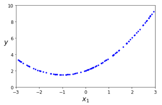
If we use X to calculate another dimension, Y, according to the quadratic formula, then we get a parabola.

y = 0.5 * X**2 + X + 2

This is not what the book did, but I am a bit stubborn trying out things.

The book added noise to this. They added a random value that is moving each point up and down by a maximum of -1 to +1.

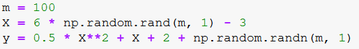
This gives the same result as in the book. Well, almost. I had not reset my random seed here. Later I fixed that.

So this is our test data. Now we need to find a line that fits this. They accurately point out that a straight line is not a good option.

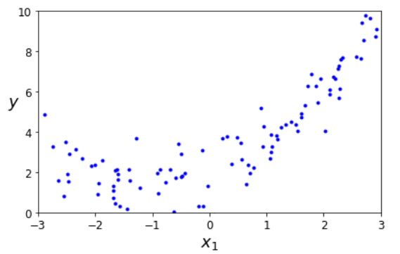
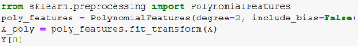
Here we create the poly_features object ready for polynomial functions of degree 2. The documentation of the PolynomialFeatures says this:

"Generate a new feature matrix consisting of all polynomial combinations of the features with degree less than or equal to the specified degree. For example, if an input sample is two dimensional and of the form [a, b], the degree-2 polynomial features are [1, a, b, a^2, ab, b^2]."

I suppose that X_poly is the result of fitting our random data to a curve. Is it not fascinating that it can do that with the X values only? The y-values are in another array. The x and y are not paired together, so how are they doing this?

The result of X_poly is an array with one hundred rows where each row has two numbers.

fit_tranform is described as follows: "Fits transformer to X and y with optional parameters fit_params and returns a transformed version of X.". Could have said blah blah. I got an uninformative book. I search for more information at the official scikit learn site and get an uninformative search result.

My best guess is that fit_transform is a general form of function. This particular object PolynomialFeatures got specific handling of the fit_transform.

https://stackoverflow.com/questions/31572487/fitting-data-vs-transforming-data-in-scikit-learn

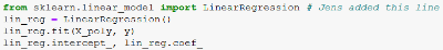
Then we go back to the linear regression.

Here I had a little intermezzo with the book because the import of LinearRegression was missing on page 125. It appeared without being imported and also in the document on Git.

https://github.com/ageron/handson-ml/blob/master/04_training_linear_models.ipynb

It had been added on page 112 in the book. While figuring this out, I also reset my random seed value the same way as the author did so that my curve started to look identical.

LinearRegression is a useful function. I found more information about it on this site: https://realpython.com/linear-regression-in-python/

Great and not great. I just want to know what the book is talking about. To find out, I pull up perhaps a 40 pages document from the Internet. I don't know how many pages since I decided I would not download that paper. You had to make an account to get hold of it, and I was not up for that tonight.

I suppose the line in the code where fit is called. That is where the linear regression object is finding a fitting curve for the data provided?

Or perhaps was that already done in the fit_transform of the polynomial function? I can as well admit I am totally clueless. I just want to bang this book on the wall. It is so bad.

The optimal weights are calculated for doing the fitting. I know that programming is often juggling several balls at the same time, but here the book is using the polynomial functionality and linear regression in between. It is confusing if you are not used to this math and Python.

 

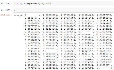
Nevertheless, I will try to explain this to myself, step by step. The first step is linspace, producing evenly spaced numbers calculated over a specified interval. It looks like this in the book:

I tried doing the same by myself to see what is coming out of these functions.

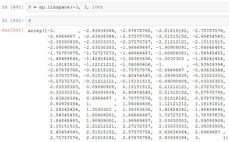
One hundred numbers evenly spaced number from -3 to +3. Then reshape(100,1) creates an array with one hundred rows where each row is an array with one element. I am wondering about the role of this array.

Next up, we use the object poly_features. It was created earlier on with input that it should handle degree=2 and include_bias was false. I suppose the object is ready for second-degree polynomials. It has the method transform, and we use that on our one hundred evenly distributed numbers.

Next, we are using our linear regression object. It was created to fit the X_poly and y. X_poly was our test data.

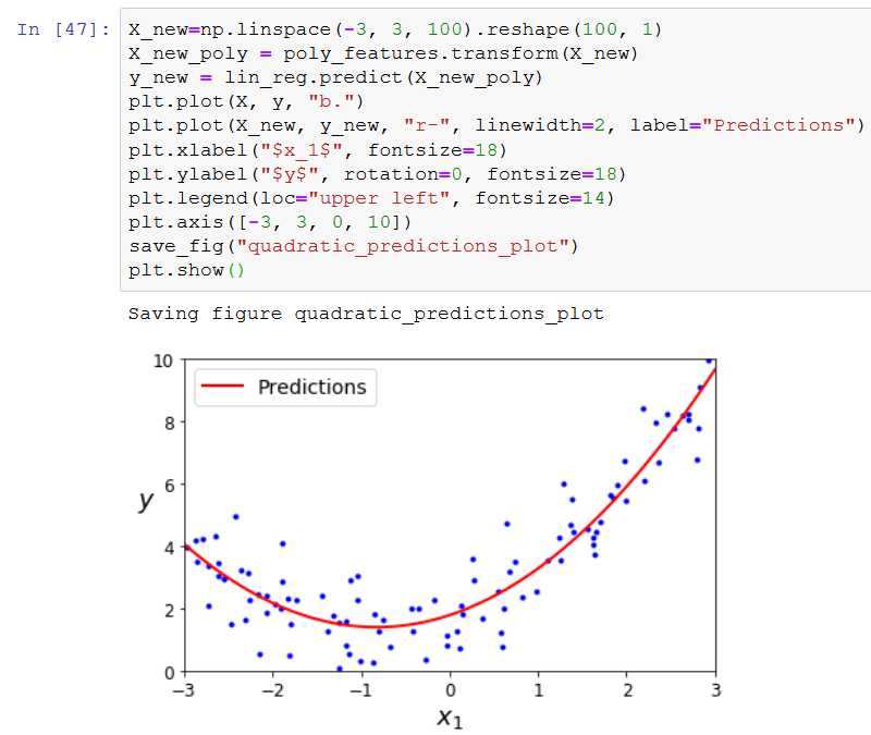
Next, we plot blue dots for X and y. That is our original test data.

Then we plot a red line of X_new and y_new, giving it the label Predictions.

I have seen this source code now, but I cannot recreate this in any way.

The conclusion so far is that the test data here is random or at least created with randomness. Then with some type of model, we can draw a line or a curve through the test data. That line or curve is a prediction. From here on, the book will divide the test data into two parts where one part is used to create our model, the prediction, and the other part is used to verify how precise the model is. The model creation part can be bigger or smaller.

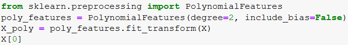
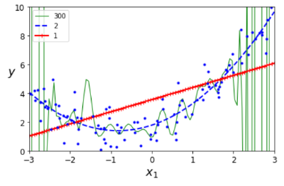
Somewhat confused and slightly annoyed, I arrived at page 125. On the next page, they explain that getting the degree right is vital for proper behavior. Using a too low degree, you get a line while it should have been a curve. A higher degree fits the curve. Much higher degree and the fitting starts wiggling around to fit as much as possible. This kind of spatial reasoning is good for me, I can grasp the gist of that. There is a code example of this reasoning producing a graph.

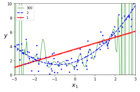
The blue dots are our data. The red line is the linear fit. The Blue striped line is the polynomial of the second degree, and the green is of degree 300. The green line is very wiggly.

When searching for the term cross-validate on my blog, I find I wrote about it in https://www.malmgren.nl/post/2019-09-03-ML-AI-Part1 on 25 August. There I say it was on page 69. I talked about it again on 2 September.

On page 127, we start to look at how to do this. There is a rule of thumb presented here:

1. If a model performs well on the training data but generalizes poorly according to the cross-validation metrics, then the model is overfitting. Cross-validation allows us to get an estimate of the performance of our model and also how precise it is, its standard deviation (page 71).
2. If it performs poorly on both, then it is underfitting.

Here we split the data. In the code example, 20 percent is split off to be used as test data (test_size=0.2), and the rest is validation values.

The way we calculate the error is by taking the distance from the data to the fitted curve (prediction), or rather it is calculated with Root Mean Square Error function described on page 37.

There is a code example on page 127 that takes a model, and it splits the data. It is a cool function. In other words, it is hard to understand what it is doing without pulling it apart. I will not do that.

Wednesday 1 January 2020

It is the first day of the year! I decided to work on the book Hands-On Machine Learning with Scikit-Learn & TensorFlow by Aurélien Géron. In this series of blog posts, you can also find news about how it is going with our house. Yesterday evening on the last day of the year 2019, I blogged about Anna, and I signed a contract with the housebuilder of the building of our house. We still need to get the mortgage finished. It is progressing well but slowly. My wife is now a secretary on the board of the road association. So that was about the house for this time. Now over to the book.

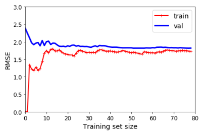
On page 127, we are using the LinearRegression, and we are using different sizes of training sets and validation sets. So I would guess that if the training set was small, the result would not be great.

So here we use a linear fitting. It is not so good for this data. When we use a ten-degree polynomial model, what happens then? The error on the training data is lower, and there is a gap between validation and training. Training data had fewer errors than the validation data. This means the model is overfitting.

Look, I learned something. That is not bad! With that conclusion, I go to bed.

Thursday 2 January 2020

It is Thursday, and it is the first regular working day of the year.

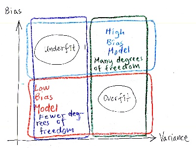
On page 129, the book talks about bias versus variance tradeoff. I think Aurelién is good at the theory, but he is not good at explaining. My theory on this has to do with that he is too intelligent. He learns stuff too easily, and then he is biased into believing that others learn this easy too. As a result, he skips essential steps in his explanations for people not as intelligent as he is.

Here he is similarly using the word bias. It is the term for wrong assumptions. "People learn very easily because I (Aurelién) learn easy," but in reality, people don't. In reality, they would like to smack his book on the wall due to frustrations. High bias in this context is that the writer assumed that his audience is much more intelligent than it is. Had he taught about the subject of his book, he might have a better understanding of how his material is received, and that would lower his bias.

The generalization error is expressed as the sum of three different types of errors:

Variance is the level of difference between people reading Aurelién's book. Some are really smart, and some are really dumb like me (apparently). A model with many degrees of freedom has a high variance. If the book is used only as a curriculum at a university, then there are fewer degrees of freedom, and the variance is lower.

Irreducible error is due to the noisiness of the readers. Some write blogs, and some don't. The only way to reduce this part is to clean up the data, fix broken sensors, or detect and remove (out)liers.

Increased model complexity increases variance and reduces bias, and vice versa reducing the model's complexity increases its bias and reduces its variance.

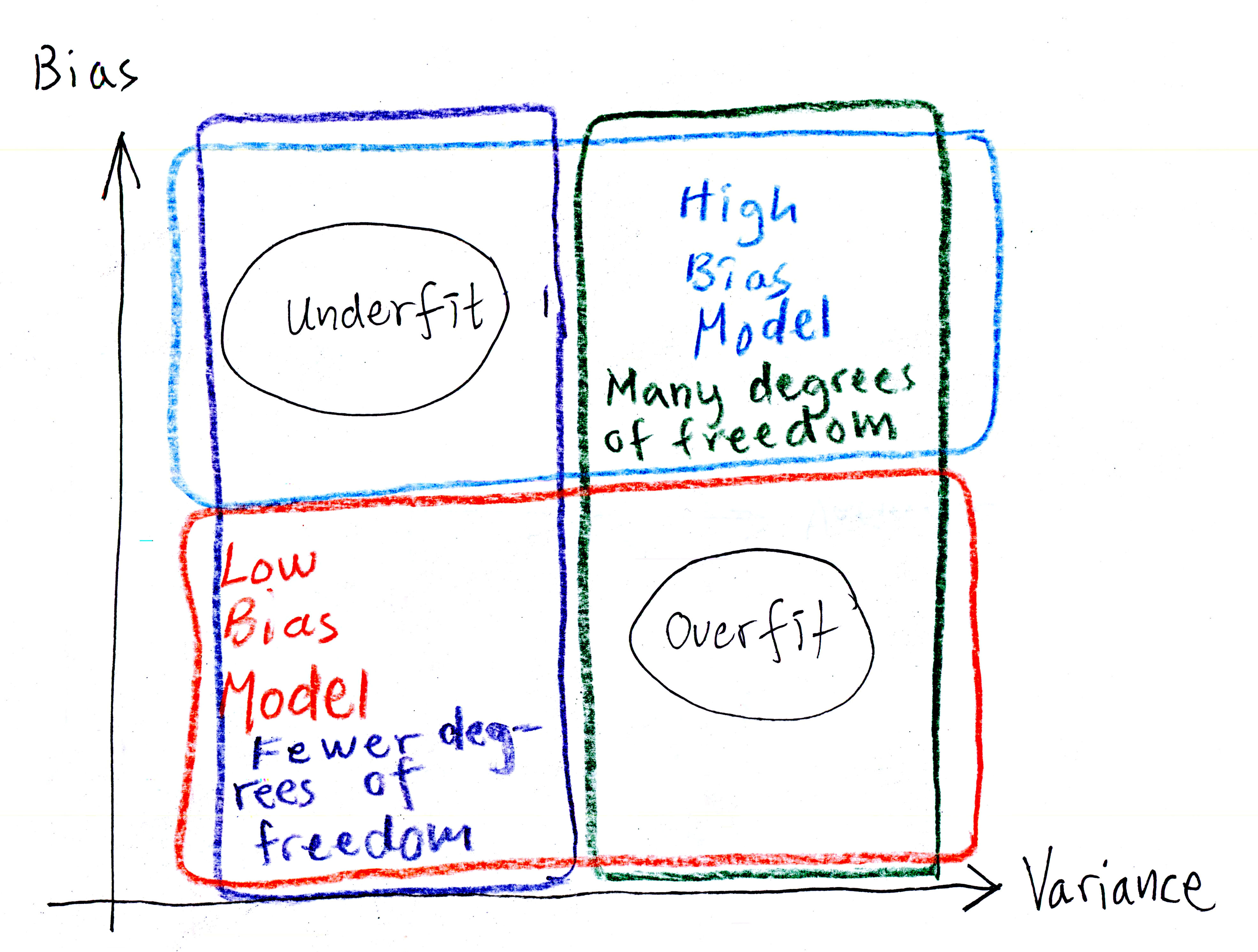
I scribbled a graph of what I think Aurelién is saying.

Time for bed.

Friday 3 January 2020

It is Friday. I am on page 130. From here on, we will explore how to reduce overfitting with different models. The process is called regularization. Here theta_i is the unregularized bias term. The added term should only be added during training. During the evaluation, there is no extra cost term added.

Linear model:	RidgeRegression	LassoRegression	Elastic Net
Also called:	Tikhonov Regression.	Least Absolute Shrinkage and Selection Operator Regression.	The middle ground between Ridge and Lasso.
Regularization term added to the cost function:	alpha times 1/2 times sumni=1 of theta2i	alpha times sumni=1|thetai|	r times alpha times sumni=1|thetai|+((1-r)/2) times a times sumni=1 of thetai2
Role of Alpha and r.	Alpha gives how much regularization to apply.	Alpha gives how much regularization to apply, but it uses smaller values than Ridge.	When r=0, then it is equal to Ridge. When r= 1, then it is equal to Lasso.
Scaler?	The data needs to be scaled using a StandardScaler.	Useless features are "automatically filtered."
	Perform Ridge Regression either with closed-form equation or gradient descent.	Use gradient descent (witch subgradient vector g15) On page 39, we can see that this is a vector because it is lowercase bold. For the rest, I don't know what this is.

 

Saturday 4 January 2020

It was great to look at the three different regularization methods yesterday and compare them. It did not lose myself on the source code, but instead, I concentrated on the text. That was great. When I go back to the source code and look at it, I feel like I can skip that part. I cannot actually skip anything, but I need to keep a good pace. In general, a model is imported, it is initialized. Then fit is called and after that predict, and the result is an array of numbers. Those numbers are not saying anything to me. It could be totally different numbers, I would not know.

Next up is early stopping on page 136. Here is a method explained that stops training as soon as the validation error reached a minimum. Between underfitting and overfitting, there is a sweet spot with a minimum amount of errors. It makes sense to stop there. Next. Oh, wait. With Stochastic and Mini batch Gradient Descent, the curves are not smooth. That makes it hard to find the sweet spot. I think moving average or going back and forth. Solvable challenge. Next.

Logistic regression on page 137. Oh uh. Now we left the regularization topic. Did we? Are we in the regression topic? Hallo Aurelién, how do we jump from regularization to classification without a gentle transition?

So, ok. Logistic regression can also be used for classification. Great. Thanks for the info.

Ah, now I see that the header Logistic Regression is of font size 18 while Early Stopping is font size 14, and that means we ended the section about regularization.

Logistic regression is also called Logit Regression.

On my blog, I have not yet implemented a math formula presentation, and I will try to defer doing that as long as possible. It had been nice, though, if it was easy to present complex math formulas here on this blog, but no.

Shall we talk about the hat for a moment? In the definitions section, on page 39, of the book, the writer introduce the notation of the hat, and it comes in something that I guess is a statistical context? He says that hat on a variable means it is a predicted value. Furthermore, he says he is using an italic font for scalar values. Lowercase bold for vectors. Uppercase bold for matrices. Yeah, cool, then that is clear. Since I cannot put a hat on a variable with my blog system, I add the text "hat" after it. Okay?

The equation 4-13 for the Logistic Regression is:

p hat = h_theta(x)=sigma(theta^Tx)

I just barely understand this. I find it hard to see if theta is written with bold or not. I feel that my knowledge that I gathered at the Khan Academy last year is wearing off. There is a graph, though, that makes sense. It is an S-shaped curve where for negative value t, the curve is planar, and the output is 0, and when t is 0, then the output increases and is at its fastest increase and at greater positive values of t, the curve is planning out again.

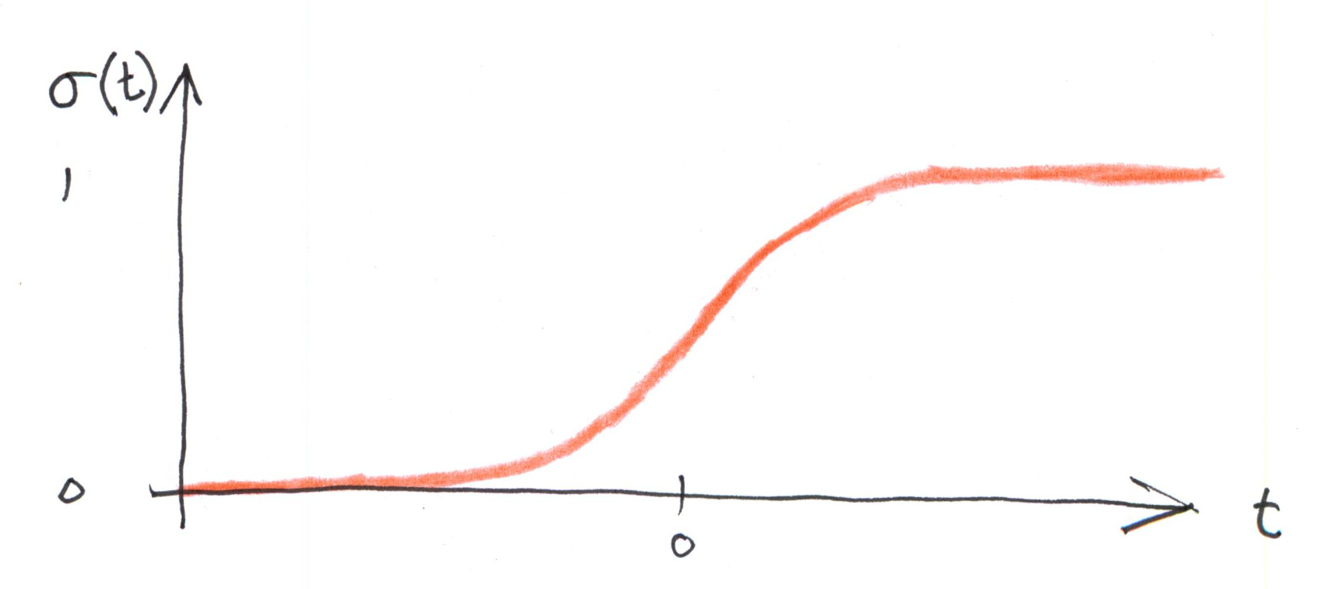
I got a hunch this function will come back again and again. The equation 4-14 for the logistic function is:

sigma(t) = 1 / (1 + exp ( -t))

Sunday 5 January 2020

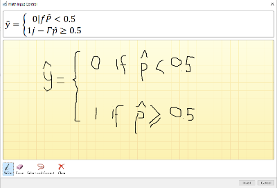
I am on page 138, and I am reading about the Logistic Regression model. I am just about to understand the equation 4-15. Would it not be nice to be able to enter it here. I tried the equation environment in Microsoft Word for the first time.

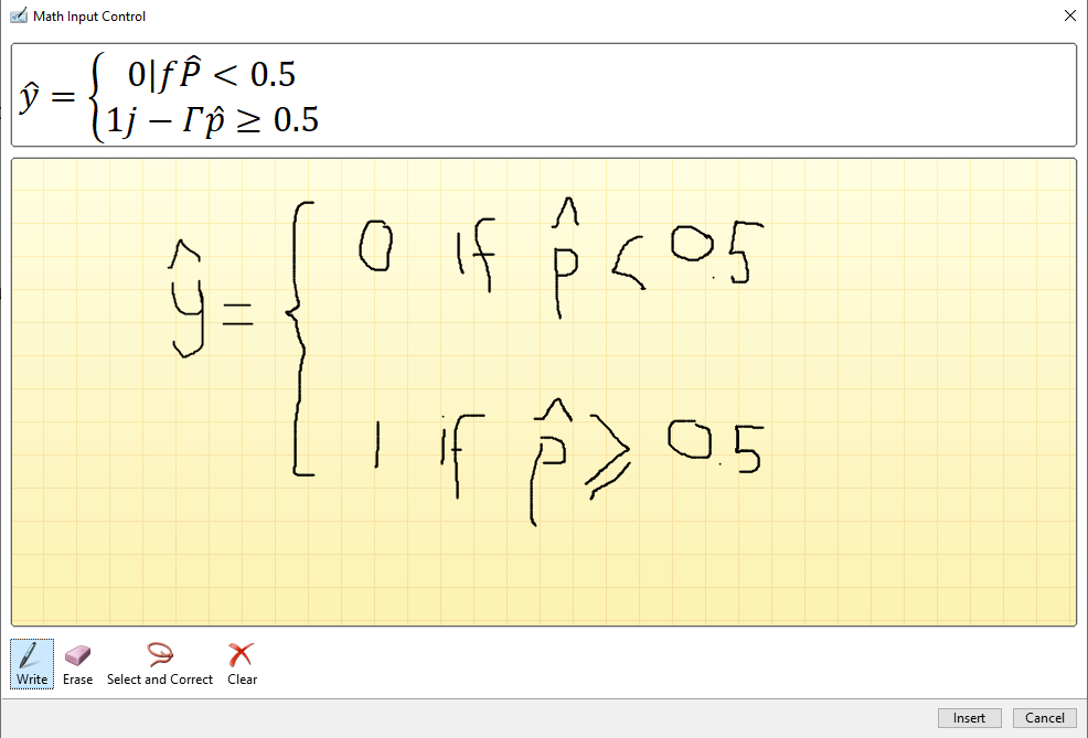
That did not go well.

Look, I managed to enter the equation 4-15 "manually."

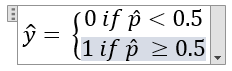
So there is an equation environment in Word, and for HTML, there is a representation in XML accepted by most web browsers. Now it is just a question about getting from one to another. But that is not for today.

So first, we need to estimate the probability p hat = h_theta(x). Here x is lowercase bold x. That means that x is a vector. With that, we can easily (although for me, nothing looks easy right now) make predictions based on the equation I have been drawing here.

Change of pace...

I am now at the end of page 138, and this book experience is becoming more and more depressing. Instead of putting the book away, I will start to read it much faster and less thorough. I will do this until I reach the second part of the book about TensorFlow. That is on page 231. I will continue to blog about the book, but there will be no testing of code examples. That takes me too much time.

We were at the Logistics Regression. If I were to summarize it, I would say that we are still working in a two-dimensional world so far. The data is given as points in an x and y-axis. The prediction is about finding some kind of curve in the data. On page and onwards, the book is talking about the classification of iris plant species. A plant is, for example, an Iris-Verginica, or it is not. Two classes at most.

On page 142, Softmax Regression. It can support several classes simultaneously.

On page 147, That went fast! Support Vector Machines. It can do linear, nonlinear classification, regression, and outlier detection. This makes me recall I started on a table back in part 2 on 11 September 2019.

Classifier	Can handle multiple classes directly	Is a strictly binary classifier	Scalability	Preferred Multiclass Method	Time Complexity	Kernal	Talked about in Jens blog
Random Forest Classifier	Yes			n/a			Part 2
Naive Bayes Classifier	Yes			n/a			Part 2
Support Vector Machine Classifier		No	Scales poorly on larger datasets	OvO	O(m2n) to O(m3n)	Yes	Part 2
Linear SVM Classifier		Yes		OvR	O(mn)	No	Part 2
SGD Classifier		Yes		OvR	O(mn)	No	Part 2
Logistic Regression		Yes					Part 4
SoftMax Regression	Yes, mutually exclusive classes.						Part 4

OvO = OneVsOneClassifier, OvR = OneVsRestClassifier

Page 147, Linear Support Vector Machine Classifier. Classes are separated with straight lines. There can be lines with margins as well. This could theoretically be a plug-in for the SVM kernel discussed next, but since this is optimized for linear solutions, it goes on its own.

Page 151, Non-Linear Support Vector Machine. This appears to be a 2D model. Areas of different classes are separated with the help of different plug-in subsystems for additional classification features:

• Polynomial kernel to express class boundaries with curves.
• Similarities features. Landmarks are specified, and around the landmark are areas defined.
• You can add a Gaussian Radial Basis Function (RBF) for class boundaries. This kernel is capable of defining classes as irregularly shaped blobs.
• There are string kernels used for classification of string subsequences
• String kernel classification based on Levenstein string distance.

Page 156, Computational Complexity. Added this to the table.

SVM Regression. This is difficult. Don't understand.

Page 158. Here the book is changing the convention for how to organize the model parameters, theta, etc. From here on, the bias will be b, and the feature weights will be called w.

Page 159, we see that a linear model can be generalized to planes in a 3D space. If the test data is placed on a horizontal plane in the 3D space and there is a plane "carving" the two classes apart, then we can start to tilt that carving plane at different angles for various optimization results.

Page 161, there exists optimization methods for tilting the plane; this is called quadratic programming. I hope I will never need it.

Page 162, The dual problem. The text talks about expressing dual problems such as two problems are similar or closely related, I suppose they "behave" equally. The thing is that one of the problems might have a smaller solution, computational wise. This is a guess.

Page 163, Kernelized SVM. There is a notations note on this page. Always good to keep an eye open for those. I will need to come back to that. Did I think we already talked about the kernels of SVM? Here it is back. On the next page 164, the common kernels formulas are listed.

The book is mentioning more dimensions, how solutions are scaled up to higher dimensions, 2 to 3.

Page 169. Decision Trees. I stop here for tonight.

Monday 6 December 2020

Perhaps I got myself an overdose of artificial intelligence this weekend. It feels hard to get this thing going again this evening. My wife is attending a board meeting of the road association tonight. I cannot say so much about it, but it is much work for her. On Friday this week, we will have a new meeting with the mortgage advisors. They have good news, the plans we decided on is going well. That is that, about the house. Now over to AI.

"To understand Decision Trees, we are not going to explain anything but through some Python code at you." Thank you, thank you, I love your style Aurelén. Not.

It looks impressive, but I skip the confusing intro and start reading on page 169. This classifier is based on a decision tree. The nodes represent a stage in the decision making. It looks like at each level, there may be two answers, true or false. The example on page 170 is a binary tree.

Page 171. It is called a predictor. Up until now, we talked about classifiers. The classifiers are from here on called predictors as well as classifiers.

Page 172. The CART training algorithm in Scikit-Learn gives binary trees. ID3 can produce trees with more children.

A decision tree gives away how it makes its decision, called "White box." Later we will see Random Forest and Neural Network called "Black box" models.

Page 173. The decision tree can estimate probabilities by recording the ratio for nodes being triggered during training.

How is the CART algorithm working? This a classic example of a failing explanation. The algorithm is making use of something called purity, and what that is, is not defined upfront. There is not even a hint that it will be explained later. Purity is talked about on the next page but still not explained. There are two algorithms for purity:

• Gini impurity. Slightly faster.
• Entropy. Produce slightly more balanced trees.

The algorithm splits the training set into two subsets by searching for the purest subsets. Each subset is then slit the same way until the tree reached the maximum depth.

Page 175, you regularize the CART training with the maximum depth.

Page 177, Decision trees can also be used for Regression. Instead of predicting a class, it predicts its value.

Page 179, Decision trees on two-dimensional data sets tend to be classified with straight lines. If the data is rotated, the result is generalizing less well. Also, there is a stochastic element, so the result is slightly random.

Page 183, Next Chapter about Assemble Learning and Random Forests. Wisdom of the crowd. We can use several training predictors in an ensemble. For example, a group of Decision Tree Classifiers each on a random subset of the training set. This is called a Random Forest. This is a useful machine learning algorithm.

There are several ensemble methods. The book will cover them from page 183 until 205. I will make a sub-series of these here below indicated by Page XXX, Ensemble: YYY.

Page 183, Ensemble: Voting Classifiers.

Tuesday 7 December 2020

I continue where I was yesterday. It is possible to create a better classifier by predicting which class gets the most votes. This is called a hard voting classifier. This classifier often achieves higher accuracy than the best classifier in the ensemble. This has to do with the law of large numbers. Ensemble methods work best if the predictors are as independent as possible, using different algorithms, for example.

Page 187, Ensemble: Bagging and Pasting.

One way to make sure the classifiers are independent is to use different training algorithms. Another approach is to train with the same training algorithm but on different random (not necessarily mutually exclusive) subsets of the data.

The text initially says “different” subsets. Then later by the context, it is apparent that it is not a mutually exclusive subset that the word “different” implies. Or perhaps I am wrong. This book is full of these things. First, we are led to believe one thing, and later it turned out to be the exact opposite. It is so tiring to learn anything from this book. But we go on.

Cutting the data in chunks like this and letting different predictors learn from these chunks is called bagging. Bagging comes from bootstrap aggregating. In statistics, resampling with replacement is called bootstrapping. The term pasting is poorly outlined in the book, IMHO.

Page 189, Ensemble: Bagging and Pasting, Out-of-Bag Evaluation.

With bagging, some instances may be sampled several times for any given predictor, while others not at all. Well, look, up until this sentence, I believed that the chunks were mutually exclusive. An out of bag set is called oob. There are interesting little details about oob, but I leave that and continue.

Page 190, Ensemble: Random Patches and Random Subspaces.

It can do sampling, as well. I forgot what sampling is. Tough luck. It is not well defined. Anywhere. There can be feature sampling and instance sampling. Anyway. We move on.

Page 191, Random Forests.

A random forest is an ensemble of decision trees generally trained via the bagging method.

Page 192, Extra-Trees.

When growing trees in a Random Forest, it is possible to use a random threshold instead of the best threshold. This is called extremely randomized trees or extra trees.

Page 193, Boosting.

Originally called hypothesis boosting. An ensemble method training predictors sequentially each trying to correct its predecessor. AdaBoost is the most popular. Stands for Adaptive Boosting.

Wednesday 8 January 2020

I had a good reading pace of the book for a couple of days. That will decline now because tomorrow I will go to the first aquarelle painting gathering of the aquarelle club this year. There is not so much news for the house. It is late, so I will not be able to do so much tonight.

Page 194, Ensemble: Boosting, Ada Boost.

For AdaBoost, any classifier can be used. The result is analyzed, and then for the next step, another classifier is selected, and the mistakes of the previous classifier are used to recalculate the weights (boosted) for the next classifier.

Page 197, Ensemble: Boosting, Gradient Boosting.

Like Ada Boost, sequentially adding predictors to an ensemble. Instead of tweaking weights, it tries to fit the new predictor to the residual errors made by the previous predictor. I cannot find a concise definition of residual errors, so I leave that to the future me to find out. Or not.

Page 202, Ensemble: Stacking.

Short for stacked generalization. In previous boosting, a trivial function tried to improve the predictions with, for example, hard voting, etc. Why not train a model to carry out the aggregation and produce the final prediction? The predictor making the final prediction is called a blender.

The next chapter is dimensionality reduction. With a bit of luck, I will work on that on Friday evening. Otherwise on Saturday. For now, I go to bed.

Tuesday 14 January 2020

It is already Tuesday, and my prediction came true, I did not have much time to work on the AI book. On Thursday, I went to the aquarelle club, and on Friday evening, I was painting. That did not go so well. Also, on Friday, we had a meeting with the mortgage advisor, and that went fine. The process of finalizing the mortgage has started. It will take a week. During the weekend, I worked on an action figure, and that slipped away to Monday evening as well. Today we had a message from the building company. They will start working on the foundation before the summer at our plot. During the summer the house will be constructed in the factory. In September, they will assemble the house on our location.

So that is all about that. I am writing this on my new secondhand laptop on the train to the Swedish folk music and dance event in Amstelveen. This laptop is lovely. It will be even more fantastic when I have arranged a second sim card for it. Then I will have an internet connection everywhere. While working on the little action figure, I cut myself in my thumb. Now I made some bloodstains on page 207 at the chapter Dimensionality Reduction. To get to the folk music location, I also must travel by bus, and I could read my book on the bus as well.

Now I am on my way home. It was great. Joost was there, and others I don’t know the names of so well. There was a new young Dutch lady, Judith, that had studied music in Sweden in Uppsala.

I had to wait for the train. It was good. I had the book I was reading about dimensionality reduction. Up until now, the book presented mostly two-dimensional data. That is all well and fine, but there are also data in three dimensions and even higher dimensions. It turns out that the higher the dimensions the data has, the more it is filled with useless gaps.

It is often possible to compress useless parts of the data. It is sometimes possible to project data from a higher dimension to a form of data with a lower dimension. For example, from 3D to 2D by taking a plane from the 3D space.

Sometimes data is curled up in a higher dimension. Then it is necessary to unfold it before projecting it to a lower dimension.

Page 212. The book talks about the Manifold assumption. In most real-world high dimensional datasets lie close to a much lower-dimensional manifold. This assumption is often empirically observed. A smaller dataset is often easier and quicker to work with.

Page 213, Principal Component Analysis, PCA. Popular reduction algorithm. It is important to consider the variance when reducing the dimensions. It sounds like PCA takes slices of the data to calculate the variance, and then it selects the slice keeping most of the variance. One such slice is called a principal component.

That was it for today. It is late. Very late. I am back home.

Sunday 19 January 2020

It is Sunday morning right now, and there is a moment for reading the book. There has been a couple of days since I was working on the book, and I can feel that my brain is stuttering on the material. The sim card arrived, and it works.

Page 215, Singular Value Decomposition, SVD. There is a function in NumPy to find the SVD. When using this functionality, it is important to center the data. The book asks the reader not to forget to center the data before using SVD.

Page 215, Projecting Down to d Dimensions. I think this is a really cool feature that we are seeing here. We look at the data in different ways at the data, principal components, and we determine the variance for the various components. I suppose we sort the components based on variance, and then we decide on “keeping” the d first components. I cannot see in the book that the components are sorted, but the book does talks about keeping much variance as possible.

Monday 20 January 2020

It is already Monday! My wife and I went to the municipality to sign the purchase contract for the plot. Wit that the municipality started the process of letting the notary pass the purchase, as it is called. That will happen in four weeks from now. The road association has worked hard. Unfortunately, it is not going so well with the electricity and waterside of the road project. The physical road will be finished quicker, but it will take a long time before we get electricity, water, and the Internet. It all depends on various scenarios. The worst case is a year from now. Perhaps off-grid life is something we will try out a little. We are planning on 24 solar panels, so there is potential.

Back to the book, page 217. The question is, how many dimensions to keep. For this, they introduce the term, explained variance. It takes into account how much of the data is lying within a component. Then it is possible to plot the dimensions, the components, sorted such that the dimensions, including most data, come first and then further away come the dimensions of lesser data. This forms a curve that starts steep upwards and then becomes less and less steep. It is possible to spot an ideal place to cut.

Page 218, PCA for compression. It is possible to reverse PCA to generate something similar to the original data. It sounds like magic.

Here I jump to page 223, LLE. Locally Linear Embedding. This is a non-linear dimensionality reduction technique, NLDR.

Friday 31 January 2020

It is Friday, and I had a too-long pause from the book. This is not feeling good. In the meantime, I have been working a lot on 3D printing for the past two weeks. First, I printed an object for a colleague, and then I helped my daughter with an assignment for school. She is studying architecture at the university. That latter was a huge assignment, and I helped her, and she got a pretty good score.

I wish my relationship with this book was better. We are getting along. That is more or less it.

Page 225. Other Dimensionality Reduction Techniques.

• Multidimensional Scaling.
• Isomap.
• T-Distributed Stochastic Neighbor Embedding (s-SNE).
• Linear Discriminant Analysis.

And that is it. We reached the end of part one of the book.

At the end it was feeling less and less motivating to read the book.